딥러닝 모델 만들기

전처리 (colab 이용)

from google.colab import drive
drive.mount('/content/drive')

DATA_PATH = "/content/drive/MyDrive/"
DATA_PATH

SEED = 42

import torch
import numpy as np

# 시드 고정을 위해
import random 
import os

import pandas as pd
from sklearn.preprocessing import OneHotEncoder
from sklearn.model_selection import train_test_split
from sklearn.model_selection import cross_val_score
from sklearn.model_selection import KFold

# titanic 데이터셋 사용
>>> df = pd.read_csv(f"{DATA_PATH}titanic_train.csv")

결측치 미리 채우기

# age 중앙값
>>> df.age = df.age.fillna(df.age.median()) 

# fare 중앙값
>>> df.fare = df.fare.fillna(df.fare.median())

# cabin 임의의 문자열로 채우기
>>> df.cabin = df.cabin.fillna("UNK")

# embarked 최빈값
>>> df.embarked = df.embarked.fillna(df.embarked.mode()[0]) 

# 학습에 바로 사용가능한 특성
>>> cols = ["pclass","age","sibsp","parch","fare"]
>>> features = df[cols]

범주형 one-hot encoding

>>> cols = ["gender","embarked"]
>>> enc = OneHotEncoder()
>>> tmp = pd.DataFrame(
>>>     enc.fit_transform(df[cols]).toarray(),
>>>     columns = enc.get_feature_names_out()
>>> )

# 특성
>>> features = pd.concat([features,tmp],axis=1)

# 정답값
>>> y_train = df["survived"].to_numpy()

스케일링

>>> from sklearn.preprocessing import MinMaxScaler
>>> scaler = MinMaxScaler()
>>> x_train = scaler.fit_transform(features)

>>> x_train.shape , y_train.shape
((916, 10), (916,))

재현성 함수 (Reproduction)

동일하게 학습되지 않는다 = 예측 결과가 보장되지 않는다 = 재현성이 보장되지 않는다
재현성 함수를 돌림으로써 어느정도의 재현성 보장
형식이니까 외워라

>>> def reset_seeds(seed):
>>>     random.seed(seed)
>>>     os.environ['PYTHONHASHSEED'] = str(seed)
>>>     np.random.seed(seed)
>>>     torch.manual_seed(seed)
>>>     torch.cuda.manual_seed(seed)
>>>     torch.backends.cudnn.deterministic = True  
    
    
>>> reset_seeds(SEED)

데이터셋 클래스 만들기

>>> class TitanicDataset(torch.utils.data.Dataset):
>>>     def __init__(self,x,y=None):
>>>         self.x = x
>>>         self.y = y

			# 정답 데이터도 같이 들어왔을 때 2차원 형태로 만들어주자
>>>         if self.y is not None:
>>>             self.y = y.reshape(-1,1)

>>>     def __len__(self):
>>>         return self.x.shape[0]

>>>     def __getitem__(self,idx):
>>>         item = {}
>>>         item["x"] = torch.Tensor(self.x[idx])
>>>         if self.y is not None:
>>>             item["y"] = torch.Tensor(self.y[idx])
>>>         return item

>>> train_dt = TitanicDataset(x_train,y_train)

>>> train_dl = torch.utils.data.DataLoader(train_dt,batch_size=2,shuffle = False)
>>> train_dl
<torch.utils.data.dataloader.DataLoader at 0x7ff3faa2b6a0>

>>> data = next(iter(train_dl))
>>> data
{'x': tensor([[0.0000, 0.8873, 0.0000, 0.0000, 0.0966, 0.0000, 1.0000, 1.0000, 0.0000,
          0.0000],
         [1.0000, 0.4238, 0.0000, 0.0000, 0.0157, 0.0000, 1.0000, 0.0000, 0.0000,
          1.0000]]),
 'y': tensor([[0.],
         [0.]])}

torch.nn.Linear 레이어

입력받은 데이터를 선형 변환 해주는 레이어
fully connected layer 라고도 한다

>>> reset_seeds(SEED)

>>> hidden_layer = torch.nn.Linear(x_train.shape[1],4)
>>> x = hidden_layer(data["x"])
>>> x
tensor([[ 0.3429,  0.2720, -0.2034,  0.3389],
        [ 0.0509,  0.5410, -0.4339,  0.4020]], grad_fn=<AddmmBackward0>)

활성화 함수 (Activation function)

입력된 데이터의 가중 합을 출력신호로 변환하는 함수

시그모이드 함수 (Sigmoid)

0 ~ 1 사이의 값을 가지는 함수

>>> sig = torch.nn.Sigmoid()
>>> sig(x)

tensor([[0.5849, 0.5676, 0.4493, 0.5839],
        [0.5127, 0.6320, 0.3932, 0.5992]], grad_fn=<SigmoidBackward0>)

탄젠트 함수 (Hyperbolic Tangent)

-1 ~ 1 사이의 값을 갖는 함수

>>> tanh = torch.nn.Tanh()
>>> tanh(x)

tensor([[ 0.3301,  0.2655, -0.2006,  0.3265],
        [ 0.0509,  0.4937, -0.4086,  0.3817]], grad_fn=<TanhBackward0>)

ReLU (Rectified Linear Unit)

입력이 0 이상이면 입력을 그대로 출력하고, 음수이면 0을 출력
Dying relu 현상 (노드가 죽는 현상)이 발생하는 문제가 있다
비선형성이 추가됨

>>> relu = torch.nn.ReLU()
>>> relu(x)

tensor([[0.3429, 0.2720, 0.0000, 0.3389],
        [0.0509, 0.5410, 0.0000, 0.4020]], grad_fn=<ReluBackward0>)

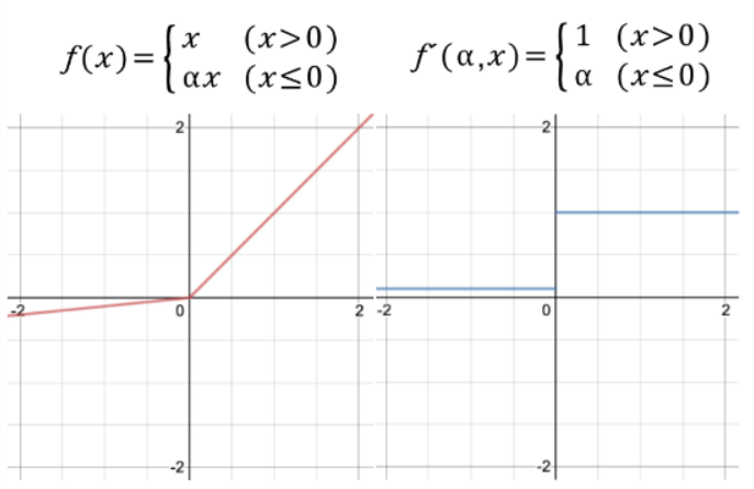
Leaky ReLU

ReLU의 변형된 함수
Dying ReLU 현상을 해결하기 위해 나온 함수

>>> lk_relu = torch.nn.LeakyReLU()
>>> lk_relu(x)

tensor([[ 0.3429,  0.2720, -0.0020,  0.3389],
        [ 0.0509,  0.5410, -0.0043,  0.4020]], grad_fn=<LeakyReluBackward0>)

PReLU (Parametric ReLU)

Leakly ReLU와 유사하지만 음수 입력에 대한 경사를 학습을 통해 업데이트 함

>>> p_relu = torch.nn.PReLU()
>>> p_relu(x)

tensor([[ 0.3429,  0.2720, -0.0508,  0.3389],
        [ 0.0509,  0.5410, -0.1085,  0.4020]], grad_fn=<PreluKernelBackward0>)

ELU (Exponential Linear Unit)

입력이 0 이하일 경우 지수 함수를 이용하여 부드럽게 깎아준다
exp를 계산하는 비용이 발생함

>>> elu = torch.nn.ELU()
>>> elu(x)

tensor([[ 0.3429,  0.2720, -0.1840,  0.3389],
        [ 0.0509,  0.5410, -0.3520,  0.4020]], grad_fn=<EluBackward0>)

소프트맥스 함수 (Softmax)

입력받은 값들을 출력으로 0 ~ 1 사이의 값들로 모두 정규화 하며, 출력값들의 총합은 항상 1이 되는 특성을 가짐

>>> softmax = torch.nn.Softmax(dim=1)
>>> softmax(x)

tensor([[0.2852, 0.2657, 0.1651, 0.2840],
        [0.2142, 0.3496, 0.1319, 0.3043]], grad_fn=<SoftmaxBackward0>)
        
>>> softmax(x).sum(dim=1)
tensor([1.0000, 1.0000], grad_fn=<SumBackward1>)

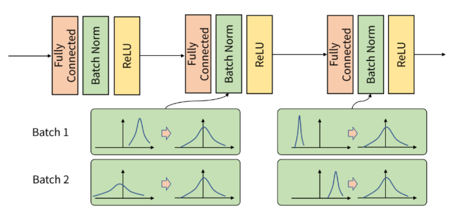
배치 정규화 (Batch Normalization), 노멀리제이션

배치 단위로 평균과 분산을 이용해 정규화
학습속도 향상
경사가 사라지거나 폭발하는 문제를 완화

>>> x
tensor([[ 0.3429,  0.2720, -0.2034,  0.3389],
        [ 0.0509,  0.5410, -0.4339,  0.4020]], grad_fn=<AddmmBackward0>)
        
        
>>> bn = torch.nn.BatchNorm1d(x.shape[1])
>>> bn(x)
tensor([[ 0.9998, -0.9997,  0.9996, -0.9950],
        [-0.9998,  0.9997, -0.9996,  0.9950]],
       grad_fn=<NativeBatchNormBackward0>)
       
       
>>> bn(x).mean(), bn(x).var()
(tensor(2.2352e-07, grad_fn=<MeanBackward0>),
 tensor(1.1395, grad_fn=<VarBackward0>))

Dropout

신경망에서 은닉층의 각 노드에 대해서 (각 노드별) 0 ~ 1 사이 확률로 랜덤하게 0으로 대체
빠른 학습 (계산 비용이 작아짐)
과대 적합 방지

>>> x
tensor([[ 0.3429,  0.2720, -0.2034,  0.3389],
        [ 0.0509,  0.5410, -0.4339,  0.4020]], grad_fn=<AddmmBackward0>)
        
        
>>> dropout = torch.nn.Dropout(0.3)
>>> dropout(x)
tensor([[ 0.0000,  0.3886, -0.2905,  0.4841],
        [ 0.0727,  0.7728, -0.6198,  0.5743]], grad_fn=<MulBackward0>)

torch.nn.Sequential

입력 텐서가 순차적으로 layer에 통과할 때 사용

>>> seq_layer = torch.nn.Sequential(
>>>     torch.nn.Linear(x_train.shape[1],8),
>>>     torch.nn.ReLU(),
>>>     torch.nn.Linear(8,4),
>>>     torch.nn.ReLU(),
>>>     torch.nn.Linear(4,1)
>>> )
>>> seq_layer

Sequential(
  (0): Linear(in_features=10, out_features=8, bias=True)
  (1): ReLU()
  (2): Linear(in_features=8, out_features=4, bias=True)
  (3): ReLU()
  (4): Linear(in_features=4, out_features=1, bias=True)
)


>>> seq_layer(data["x"])
tensor([[0.2635],
        [0.2953]], grad_fn=<AddmmBackward0>)

신경망 모델 만들기

>>> class Net(torch.nn.Module):
>>>     def __init__(self,in_features):
>>>         super().__init__()
>>>         self.seq_layer = torch.nn.Sequential(
>>>             torch.nn.Linear(in_features,8),
>>>             torch.nn.ReLU(),
>>>             torch.nn.Linear(8,4),
>>>             torch.nn.ReLU(),
>>>             torch.nn.Linear(4,1)
>>>         )

>>>     def forward(self,x):
>>>         return self.seq_layer(x)

>>> model = Net(x_train.shape[1])
>>> model(data["x"])

tensor([[-0.2592],
        [-0.2592]], grad_fn=<AddmmBackward0>)

모델 구조 보기

torchsummary

첫번째 인수로 모델 객체를 전달
input_size 파라미터: 피처 갯수를 튜플로 전달
device 파라미터: "cuda" or "cpu"

>>> import torchsummary

>>> torchsummary.summary(model,input_size=(x_train.shape[1],),device="cpu")
----------------------------------------------------------------
        Layer (type)               Output Shape         Param #
================================================================
            Linear-1                    [-1, 8]              88
              ReLU-2                    [-1, 8]               0
            Linear-3                    [-1, 4]              36
              ReLU-4                    [-1, 4]               0
            Linear-5                    [-1, 1]               5
================================================================
Total params: 129
Trainable params: 129
Non-trainable params: 0
----------------------------------------------------------------
Input size (MB): 0.00
Forward/backward pass size (MB): 0.00
Params size (MB): 0.00
Estimated Total Size (MB): 0.00
----------------------------------------------------------------

torchinfo

첫번째 인수로 모델 객체 전달
두번째 인수로 배치 사이즈와 피처 갯수를 튜플로 전달

!pip install torchinfo

>>> import torchinfo
>>> torchinfo.summary(model,(32,x_train.shape[1]) )

==========================================================================================
Layer (type:depth-idx)                   Output Shape              Param #
==========================================================================================
Net                                      [32, 1]                   --
├─Sequential: 1-1                        [32, 1]                   --
│    └─Linear: 2-1                       [32, 8]                   88
│    └─ReLU: 2-2                         [32, 8]                   --
│    └─Linear: 2-3                       [32, 4]                   36
│    └─ReLU: 2-4                         [32, 4]                   --
│    └─Linear: 2-5                       [32, 1]                   5
==========================================================================================
Total params: 129
Trainable params: 129
Non-trainable params: 0
Total mult-adds (M): 0.00
==========================================================================================
Input size (MB): 0.00
Forward/backward pass size (MB): 0.00
Params size (MB): 0.00
Estimated Total Size (MB): 0.01
==========================================================================================

내 블로그 - 관리자 홈 전환	`Q` `Q`
새 글 쓰기	`W` `W`

글 수정 (권한 있는 경우)	`E` `E`
댓글 영역으로 이동	`C` `C`

이 페이지의 URL 복사	`S` `S`
맨 위로 이동	`T` `T`
티스토리 홈 이동	`H` `H`
단축키 안내	`Shift` + `/` `⇧` + `/`

YOON-FOLIO

딥러닝 모델 만들기

전처리 (colab 이용)

재현성 함수 (Reproduction)

torch.nn.Linear 레이어

활성화 함수 (Activation function)

시그모이드 함수 (Sigmoid)

탄젠트 함수 (Hyperbolic Tangent)

ReLU (Rectified Linear Unit)

Leaky ReLU

PReLU (Parametric ReLU)

ELU (Exponential Linear Unit)

소프트맥스 함수 (Softmax)

배치 정규화 (Batch Normalization), 노멀리제이션

Dropout

torch.nn.Sequential

신경망 모델 만들기

모델 구조 보기

torchsummary

torchinfo

티스토리툴바

단축키

내 블로그

블로그 게시글

모든 영역